One of the problems with visualizations of genetic data is that it’s not always easy to incorporate spatial information. I thought about this recently in the context of trying to figure out how to deform a geographic map to reflect genetic structure (in effect, constructing a distance cartogram). The canonical multidimensional scaling approach has the disadvantage that it doesn’t preserve relative geographic positons. This is a problem because it means any transformation may not be continuous which will mean that the deformed map will not be recognisable.
SpaceMix can use geographic information as a prior, which is a start, but doesn’t guarantee that relative spatial positions will be preserved. So what we need is a constrained version of SpaceMix that preserves geographic structure. It’s not obvious how we should define that geographic structure, but I describe an example here, using the same European data that I used here. First, we take the geographic locations of the populations and construct the Delaunay triangulation of those points.
We then try to move the points around so that the distances between the points are as close to the genetic distances. Here I just use simulated annealing to minimise the difference. This is the same approach as SpaceMix - finding postions in geogenetic space for each population. To maintain geographic stricture, we make sure that the triangulation does not change - that is, each time we move a point, it has to stay within the polygon defined by the neighbouring triangles in the triangulation. We can do this efficiently by checking that the point keeps the same cross product sign with each opposite edge. This ensures that the relative positions of the points stays the same. Here’s the result, which I call Mapwarp , along with PCA and SpaceMix for comparison. The light grey lines show the triangulation.
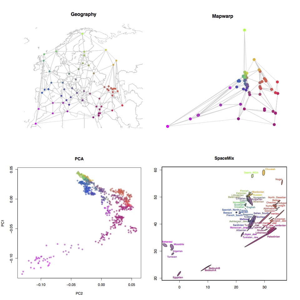
In this case, all these visualizations look quite similar - probably because the genetic structure in Europe is actually qualitatively similar to the geographic structure. That’s not always true though. A bit advantage of this approach is that the triangulation defines a mapping that allows us to deform the original geographic map to the new space. I’ll demonstrate some examples of this in another post.