More accurate ages of rare variants

###Introduction

In Mathieson & McVean (2014), Gil and I developed a method for estimating the age of \(f_2\) variants, based on the lengths of the haplotypes around them. In the paper, we used an approximation to the haplotype lengths. This note describes a slightly more accurate approximation, which we probably should have used in the first place.

###Details

####Background

Suppose two haplotypes coalesce at time \(\tau\) at their left-hand end. Then we model the distance to the next recombination event as \(\mbox{Exp}(4N_e\tau)\). So if we saw all the \(f_2\) haplotypes in a sample, then we could model the distribution of lengths as exponential, conditional on their ages. However in practice, we only see \(f_2\) haplotypes if they contain an \(f_2\) variant, which only happens if there is a mutation on the branch above the haplotype. All things being equal, this is more likely for longer haplotypes. This means that the lengths of the haplotypes are larger than would be expected under an exponential distribution.

In the extreme case, where we picked haplotypes proportional to their length, the distribution of their lengths would be \(\mbox{gamma}(2,4N_e\tau)\), or exactly twice as long. So if you pick a point on the sequence at random, the length of the haplotype you land in is twice as long as if you picked a haplotype at random. This an example of the inspection paradox.

However, the case here is actually intermediate to that, for two reasons: First because here we see a haplotype if and only if it has one or more \(f_2\) variants. The probability that this happens increases with length, but not linearly. Second, because the branches above older haplotypes tend to be longer, and therefore more likely to accumulate mutations. In the original paper, we dealt with this by modelling the lengths as gamma with shape parameter 1.5 (I call this gamma-1.5). We knew that the distribution should be intermediate to exponential (i.e. gamma-1) and gamma-2, and gamma-1.5 gave an empirically good fit. In practice this overestimates the age of more longer and more recent haplotypes, and underestimates the age of older, shorter haplotypes.

####Approximation

We can derive a more accurate approximation (which deals with the first of the two reasons above), as follows. Make the assumption that \(f_2\) mutations occur at rate \(\nu\) per unit of genetic length¹ (of course, this should really be physical length). Then, conditional on the age of the haplotype, its length has distribution with density \[ f(l;\lambda,\nu)=\lambda\left(1+\frac{\lambda}{\nu} \right)e^{-\lambda t}\left(1-e^{-\nu t}\right) \] where \(\lambda=4N_e \tau=2t\) (\(t\) is the haplotype age in generations). I don’t think that this distribution has a name. It’s not a gamma distribution, but it has the right limiting behaviour as \(\nu \rightarrow 0\) and \(\infty\), tending to \(\mbox{Exp}(\lambda)\) and \(\mbox{gamma}(2,\lambda)\), respectively². If we replace \(f_{\gamma}\) in equation 1 in the Methods of the original paper with this density, the approximation should be more accurate. Unfortunately the integral then doesn’t evaluate to something nice like the hypergeometric function but it seems to be fairly well behaved numerically. I added the function loglikelihood.age.v2 to calculate this here. You can compute it by setting v2=TRUE in MLE.from.haps and specifying \(\nu\) (confusingly named mu).

We can estimate the parameter \(\nu\) from the number of \(f_2\) variants on each of the haplotypes that we do detect. This is a positive poisson distribution with parameter \(\nu l\), and we can maximise the likelihood numerically.

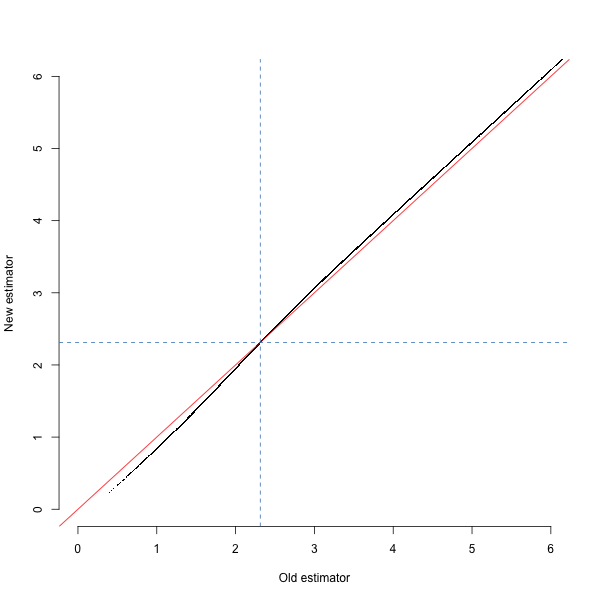
####Effect You can see the effect of the new estimate in the figure below, showing the estimated \(\log_{10}\) age of haplotypes from the 1000 Genomes GBR population under the old and new estimates. The dashed blue lines show the median - note that we chose the original approximation partly so that it would match the median value. I still need to do some simulations to show that the new estimate is actually more accurate.

####Even more accurate ages of rare variants I’m still working on improving this \(f_2\) approach. I’d like to be able to explicitly estimate split times, and also flip it round and use this approach to estimate mutation rates by seeing how the number of singletons changes with respect to the age of the haplotype. Some things that would help with this:

• Estimate \(\nu\) based on physical rather than genetic length and incorporate that into the model.

• We could also try and model the idea that \(f_2\) variants get more likely as the haplotypes get older, due to the longer branch lengths.

• Deal more accurately with the edge effects. We should incorporate the overestimate into physical length into the likelihood, particularly if we are going to estimate mutation rate. Alternatively, we could try and come up with an unbiased way of detecting the ends of the haplotypes.

####Proof Lemma: Let \(N_t\) and \(M_t\) be Poisson processes with rates \(\lambda\) and \(\mu\), respectively. Let the arrival and inter-arrival times of \(N_t\) be \(T_i\) and \(X_i\) for \(X=1\dots\) (\(T_0=0\)). Then the distribution \(X_i\) conditional on at least one arrival of \(M_t\), \(X_i|\left\{M_{T_i}-M_{T_{i-1}}>0\right\}\), is given by \[ f(x;\lambda,\nu)=\lambda\left(1+\frac{\lambda}{\nu} \right)e^{-\lambda x}\left(1-e^{-\nu x}\right) \]

Proof: Let \(A_i\) be the event that \(\left\{M_{T_i}-M_{T_{i-1}}>0\right\}\). Then, by Bayes’ rule and dropping subscripts, \[ f_{X|A}(x)=\frac{f_X(x)\mathbf{P}(A|X=x)}{\mathbf{P}(A)} \] We have \(\mathbf{P}(A|X=x)=1-e^{-\nu x}\) and

\[\begin{align} \mathbf{P}(A)&=\int_{x=0}^{\infty} \lambda e^{-\lambda x}\left(1-e^{-\nu x}\right) dx \\ &=\frac{\nu}{\nu+\lambda} \blacksquare \end{align}\]