Notes on correcting for population structure in genome-wide association studies.

Structure vs stratification

These terms are often used interchangeably but they are actually different things. Population structure refers to the actual genetic structure of the population; brought about through some kind of nonrandom mating. Stratification refers to some phenotype being correlated with the structure. That is, you could group the individuals based on clustering on genetic structure, and find that those groups were different, or stratified, with respect to some phenotype. This is what we are largely concerned about in GWAS but in fact, population structure even in the absence of stratification can still be an issue. I think there are three main types of confounding issues.

Types of confounding

Environmental stratification

This occurs when some environmental variable that affects the phenotype is correlated with the genetic structure. So the estimated genetic effects are biased because they also capture some of the environmental variation. This is probably the biggest issue for GWAS in humans.

Background genetic effects

This is when the genetic variant you are testing is correlated with other genetic variants across the genome which themselves are associated with the phenotype. One way of thinking of this is that it’s like environmental stratification, but the environment is induced by the rest of the genome. Another is to think about it in terms of LD. For example, population structure induces LD across the whole genome. This tends to be less of a concern in human GWAS, but a big problem in more heavily structured contexts.

Cryptic relatedness

This is when the individuals in your sample are not truly independent. It doesn’t bias the effect sizes, but it does mean that your standard errors are too small (effectively, you think that your sample size is larger than it actually is). This definitely tends to be something that people don’t worry about much in humans these days, but it’s certainly an issue in other contexts. See Voight and Pritchard (2005) for a nice treatment.

Types of Correction

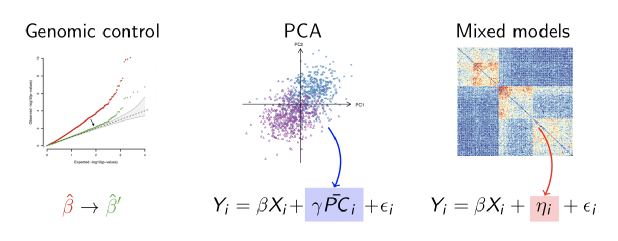
Genomic control

Introduced by Devlin & Roeder (1999) (see also 1 2) in the case-control context, this approach is basically to scale the test statistics so that they match the theoretical null distribution in some sense. The most commonly used approach is to match the median test statistic. One nice feature is that you can measure the extent of inflation in the test statistics by the genomic inflation statistic \(\lambda\) which is the ratio of observed to expected median test statistic. Genomic control effectively forces \(\lambda=1\). In simple cases, for example a case-control study with structure between cases and controls, this approach is guaranteed to produce well-calibrated test statistics although in practice that might not be the case. There are two main limitations. First, although you are guaranteed that the bulk of the distribution of test-statistics is well-calibrated, the tail of the distribution, which is the bit you care about, may not be. Details of demographic history and errors in estimating \(\lambda\) can lead to uncorrected stratification (Mathieson et al. 2012, Marchini et al. 2004). Second, in recent times genomic control has fallen out of fashion because many traits are sufficiently polygenic that with large sample sizes, we actually expect \(\lambda>1\) and genomic control might be conservative. For this reason many people have turned to LD score regression to detect confounding rather than relying on \(\lambda\). That said, in my opinion genomic control actually has a broader use than just association studies and is still useful to control for the effects of genetic drift in the calculation of any genome-wide statistic (for example, selection statistics).

Principal components

One of the original alternatives to genomic control was something called structured association, where you would cluster your structured population into hopefully homogenous groups, and run the association test separately in each group - therefore avoiding the effects of the structure. The problem with this approach was that it was difficult in practice to do the clustering, largely because most real populations exhibit continuous structure so any discrete clustering is somewhat arbitrary and does not lead to unstructured subpopulations. Instead, principal component correction infers the continuous structure and uses it, in the form of the principal components, as a covariate in the regression. Despite the necessary assumption of linear effects, in practice, this is an extremely effective was of controlling for environmental stratification, and is by far the most common approach used today.

Mixed models

The third common approach is to used mixed linear models. The standard linear model is \(\bar{Y}=\bar{X}\beta+\bar{\epsilon}\) where \(Y\) is the phenotype vector, \(X\) is the genotype vector and \(\beta\) is the SNP effect. The elements of the error vector \(\bar{\epsilon}\) are IID. In the mixed model, there is an additional term: \(\bar{Y}=\bar{X}\beta+\bar{\epsilon}+\bar{\eta}\), where the elements of \({\bar{\eta}}\) have a fixed covariance structure (usually the kinship matrix). These models originate from the animal breeding literature where the kinship matrix was originally defined by the pedigree, but in humans it is usually inferred from the data (e.g. EMMAX). In fact, it can be shown that, because the principal components are just the eigenvectors of the kinship matrix, the mixed model can be written as \(\bar{Y}=\bar{X}\beta+\bar{\epsilon}+a_1P_1+a_2P_2+a_3P_3+\dots\) where \(P_i\) are the principal components. The only difference is that in the mixed model, the likelihood of the coefficients \(a_i\) is given by a Gaussian function with variance proportional to the eigenvalue of \(P_i\), while in the standard principal component correction, the likelihood is constant. Put another way, the difference between the mixed model and PCA corrections is that the mixed model assumes that the contribution of each principal component is proportional to its eigenvalue, while the PCA correction does not.

Which correction should you use?

Depends what you are correcting for. If you are correcting for polygenic background genetic effects, it makes sense to use a mixed model, since you know that the covariance of the background effects should be equal to the kinship matrix. A special case of this is assortative mating, where the background effects are not uniformly distributed over the genome, but are precisely the regions that contribute to the variance of the trait which drives assortment. Therefore, if you know what they are, you should correct using a kinship matrix derived from those regions.

If you’re correcting for for environmental stratification, it probably makes more sense to use PCA, since there’s no reason to think that the covariance structure of those effects would be the same as the kinship matrix. Genomic control is probably conservative for very large GWAS of polygenic traits but still useful, particularly for some non-traditional study designs.